In my previous article, we discussed about rice, beans, meat and a little bit about the linear programming module of the Scipy optimize library (❁´◡`❁). It was a good introduction to the concept of optimization and was shown with an everyday scenario as an example. If you missed it, check it out here: My first optimization article.

In this article however, we would look at another python module still under the scipy library, but better applicable for more complex optimizations and I am very excited to share it with you. lets gooo!

How do we go through this exciting journey? My four-step roadmap would be:

1. Describe a Scenario

2. Explanation of the problem to be solved

3. Solving the problem using scipy.optimize minimize module

4. Review of our solution

Scenario

Now let us paint another scenario but a more technical not so everyday one.

Imagine you are a data analyst, working for a stock price forecast company and you have a historical dataset of their previous forecasts and the eventual real stock prices. You want to try to improve the forecast model already in place in this your company. The data available to you, which you’ve cleaned and organized into a data frame in python looks like this:

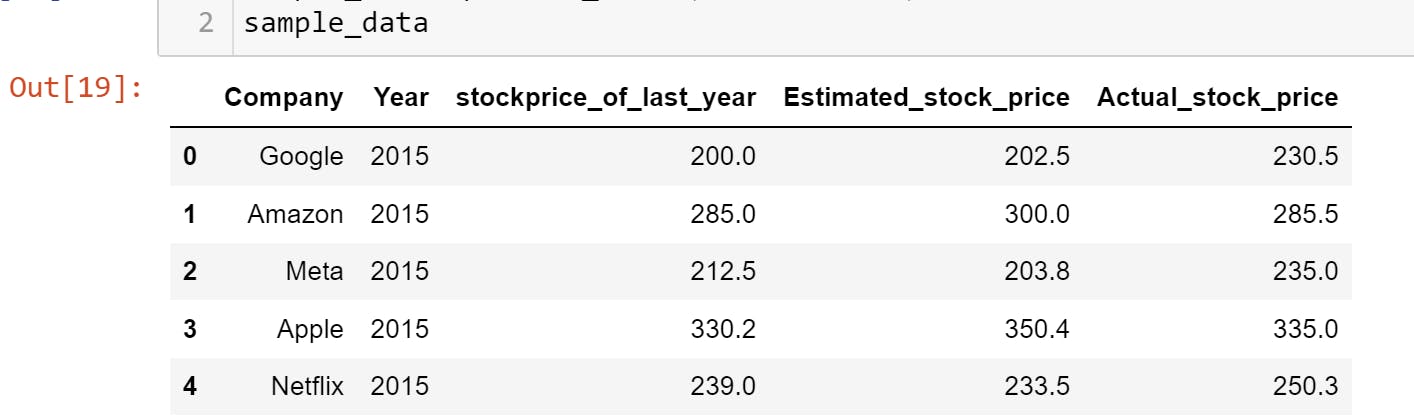
Let us also assume that in generating the estimated stock prices, your company analysts use a simple function or model :

$$P = a+l^b ........eqn1$$

where p is the estimated stock price, a and b are the input variables and l is the last year's price. (we can also assume that a must be greater than or equal to 0 and (a-b) must be greater than or equal to zero in this model) mathematically,

$$a>=0, a-b>=0 .........eqn2$$

We know, that the goal of a forecast is to get an estimated price as close as possible to the actual value. How can we use the concept of optimization then, to determine the best values of a and b that will result in an estimated stock price forcasting model that gives the closest possible value to the real stock price based on historical data?

Explanation of the problem to be solved

If we wanted to simply use optimization to get the values of a and b that would ensure the difference between the forecast price(P) and the real price(R) is minimized, The function to minimize becomes:

$$R-P$$

but, if we think a little deeper, this difference could be positive or negative and in this case, the sign of this difference does not matter since the goal is to be as close as possible to the real stock price whether higher or lower. Mathematically, by squaring this difference, we can get a value that is indifferent to the signs. for the sake of this article let us call this the absolute difference.

The real goal now, therefore, is to minimize the absolute difference between real and estimated stock prices. Also since we are dealing with a group of companies and still maintaining the same model parameters (a and b), we use the sum of this absolute difference (D). ps: if you are not really a fan of maths that much, skip these equations and look at the explanations just below them.

Thus:

$$minimize \Sigma_{i=1}^{n} (R-P)^2..........eqn3$$

where:

$$D = (R-P)^2$$

All these equations are basically saying is that we would try to minimize the total difference between our estimated and real stock prices to get the perfect values for our input variables a and b.

Now as you can see here, the linprog module (discussed in the last article) which uses the matrix of coefficients of the input variables to be minimized cannot be easily applied here without extremely complex mathematical manipulations.

Thankfully, the Scipy.optimize.minimize module comes in handy here.

Solving the problem using scipy.optimize minimize module

Remember the data we showed earlier, we can use the data frame methods to define the objective function.

My code will look like this:

#Function definition for the function to be minimized
def abs_diff(input_var):
    a =input_var[0]
    b =input_var[1]
    d = 0
    for index, row in sample_data.iterrows():
        d+=(row.Actual_stock_price- (a+(row.stockprice_of_last_year**b)))**2
    return d

Note: sample_data is the name given to the dataframe in the scenario described earlier in this article.

The above is the function to be minimized. you must define this function. (p.s: refer to python function definition if you are new to it here functions in python by freecodecamp). I used the iterrows method for pandas data frames for my code above. Here is a link to documentation for the iterrows method. However, the way we arrive at the objective function does not matter to us here, but 3 things must be in place when defining the function to be minimized. They are:

1. The input argument to the function must be (a list of) the input variables to this minimization( in this case, a and b)

2. The value to be returned must be the value we want to minimize

3. The function must contain in some way, the input variables while computing (notice that p was computed as 'a+l^b' in line 7 of the code above)

Now to the actual minimize method and how to use it. I continue my code :

import scipy.optimize as sci
bound = ((0,None), (None, None))
x0 = [0,0]
const = {'type': 'ineq', 'fun': lambda input_var: input_var[0]-input_var[1]}
result = sci.minimize(abs_diff, x0, constraints = const, bounds= bound)
result.x

line 1: we import the scipy.optimize library as we always do. Now as always, for the more technical details, refer to the documentation.

The next three lines are simply assigning values to bounds, x0 and constraints which we will explain below since they are arguments used in the minimize method in line 5.

Line 5: The minimize method is called here. The arguments are as follows:

abs_diff: This is the objective function to be minimized. It is the function we defined above in the first block of code. And it must be called first.

bound: this is a sequence of tuples for the different input variables signifying their min and max (min, max). notice that for the first input variable, a, has (o, none) beacuse from eqn2 above, a must be greater than or equal to 0.

x0: simply specifies where the function should begin its iterations from. it is your initial guess. Having used this library a few times, I can advise you to use (0, 0) most times if you are confused.

const: This is my constraint. the constraint is a dictionary specifying type(could be 'eq' for equality and 'ineq' for inequality.) fun (specifies the constraint equation). i use a lambda function in this case as it is simpler. also note: the lamda function for inequality is set at default to be a greater than or equal to.

One more argument that you could specify here is 'method': It selects the style or model used for the minimization operation. It is optional because the minimize module has selected engines based on certain conditions for any minimization operation. I would recommend not specifying if you are not sure of which method to use. For more information on the different methods see The documentation again. Scroll down to methods

result.x: this is where we call our results for the input variables.

your answer should look like this:

array([57.10791744,  0.96633564])

This tells us that using our data and model, the best value that gives us a close estimated stock price would be when a= 57.10791744 and b = 0.96633564.

It is worth noting again is that if we were to maximize, it would be the same parameters but we change the signs for the Right hand side of the objective function.

Review of our solution

To show the result of our new prediction model parameters, We use the new values of a and b to compute for new predictions on same data to see what we get.

To do this, my code:

a = result.x[0]
b= result.x[1]
sample_data['New predictions'] = a+(sample_data['stockprice_of_last_year'])**b
sample_data

The output showing the new prediction in a new prediction column is:

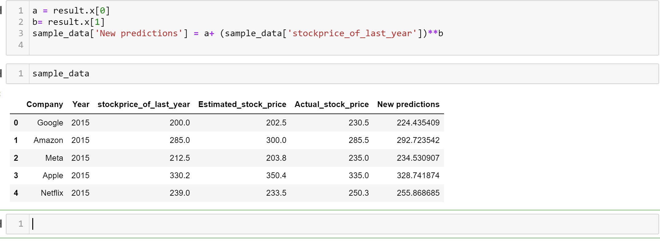
Wow! What do you see? Let me know in the comments section.

Further analysis can be carried out to show the correlation between real stock prices and our new prediction model as well as other statistical analysis which are beyond the scope of this article. However the whole point of this article has been to show clearly a useful application of one of the optimization techniques available in python.

N.B: All the data and the assumed model formula in this article is a dummy crafted in my head and does not represent any real-world information. All code here was written to teach the subject matter with little to no consideration for speed and efficiency.

Let me know if you learnt something from this. Also, I would love to hear about how relevant optimization techniques can be in your industry or business.

See you soon!